最初に

前回、ロジスティック回帰祭りで因果探索を行うという記事を書きましたが、それのつながりで、因果探索の1手法として、LiNGAMの理論に重きを置き、解説記事を書いていこうと思います。
因果探索といえば、現状因果推論の熱が高まるこの時代に、因果推論の前段階として、どこに因果がありそうなのかの探索を行うという意味で、ともに重要な分野であると思っています。なので、この次はベイジアンネットワークによる因果探索を扱う予定です。理論の部分に関しては、概念的説明も踏まえて、わかりやすくするつもりですが、数式が出てくるので、若干優しいものではなくなってしまうかもしれませんがすみません。

LiNGAM

概念的説明

LiNGAMは「Linear Non-Gaussian Acyclic Model」の略称で、変数間の因果関係を推定するための統計的手法です。この手法は、観測データから隠れた因果構造を発見することを目的としています。
LiNGAMの基本的な考え方は、観測された変数間の関係が線形で、非ガウス性（正規分布に従わない性質）を持ち、かつ循環的な因果関係を含まないという仮定に基づいています。この仮定のもと、LiNGAMは変数間の因果の向きと強さを推定します。
従来の因果推論手法と比較して、LiNGAMの特徴は非ガウス性を利用する点にあります。ガウス分布に従うデータでは因果の向きを特定することが困難でしたが、非ガウス性を仮定することで、より正確な因果推論が可能になりました。
LiNGAMの探索プロセスでは、まず観測データから変数間の統計的独立性を評価します。次に、独立成分分析（ICA）を用いて、データを互いに独立な要素に分解します。最後に、これらの独立成分から因果構造を再構築します。

理論

LiNGAMの基本モデルは以下の数式で表現されます

$x = Bx + e$

ここで

$x$ は観測変数のベクトル

$B$ は因果効果を表す係数行列（対角成分は0）

$e$ は外生変数（ノイズ項）のベクトル

この式は、各変数が他の変数の線形結合とノイズ項の和で表現されることを示しています。重要な点は、 $B$ が下三角行列（または行列の並べ替えで下三角になる行列）であることです。これは、因果関係に循環がないことを意味します。

LiNGAMの特徴的な仮定は、ノイズ項 $e$ が非ガウス分布に従うことです。この仮定により、独立成分分析（ICA）を適用することが可能になります。ICAは以下の式で表現されます

$x = As$

ここで

$A$ は混合行列

$s$ は互いに独立な非ガウス信号源

LiNGAMのアルゴリズムは、この ICA モデルを因果モデルに変換することで因果構造を推定します。具体的には、 $A^{-1}$ を計算し、その行を並べ替えて可能な限り下三角に近い行列 $W$ を得ます。この $W$ が $(I-B)$ に相当し、因果構造を表現します。

　　
LiNGAMの理論的背景には、非ガウス性を利用することで因果の向きを一意に決定できるという洞察があります。ガウス分布の場合、二変数間の関係は相関係数のみで表現され、因果の向きを特定できません。しかし、非ガウス分布では、高次のモーメントや独立性の情報を利用することで、因果の向きを推定することが可能になります。
この手法は、観測データのみから因果構造を推定できる点で画期的です。従来の手法では、介入実験や時系列データなどの追加情報が必要でしたが、LiNGAMはクロスセクショナルなデータでも因果推論が可能です。
ただし、LiNGAMにも制約があります。例えば、実際のデータが完全に線形でない場合や、重要な潜在変数が存在する場合には、推定結果が不正確になる可能性があります。また、サンプルサイズが小さい場合や、ノイズが大きい場合にも推定の精度が落ちる傾向があります。

普通のLiNGAM実装してみた

class LiNGAM:
    def __init__(self):
        # 因果順序と隣接行列を保持するための変数を初期化
        self.causal_order_ = None
        self.adjacency_matrix_ = None

    def fit(self, X):
        # DataFrameの場合はnumpy配列に変換
        if isinstance(X, pd.DataFrame):
            X = X.values
        n, p = X.shape
        
        # Step 1: データのセンタリングと白色化
        X_centered = X - X.mean(axis=0)
        cov = np.cov(X_centered, rowvar=False)
        eig_vals, eig_vecs = np.linalg.eigh(cov)
        W = np.dot(np.diag(1.0 / np.sqrt(eig_vals)), eig_vecs.T)
        X_white = np.dot(X_centered, W.T)

        # Step 2: ICAの適用
        W_ = self._fastICA(X_white)
        B = np.dot(W_, W)

        # Step 3: 因果順序の推定
        causal_order = self._estimate_causal_order(B)
        B_perm = B[causal_order][:, causal_order]

        # Step 4: スケーリングと因果効果の推定
        D = np.diag(1.0 / np.diag(B_perm))
        B_final = np.eye(p) - np.dot(D, B_perm)

        # Step 5: プルーニング
        B_final = self._pruning(X[:, causal_order], B_final)

        # 推定された因果順序と隣接行列を保存
        self.causal_order_ = causal_order
        self.adjacency_matrix_ = B_final
        return self

    def _fastICA(self, X, max_iter=1000, tol=1e-4):
        """Fast ICA アルゴリズムの実装"""
        n, p = X.shape
        # ランダムな初期の重み行列を生成
        W = np.random.randn(p, p)
        for iteration in range(max_iter):
            W_new = self._ica_iteration(X, W)
            # 収束判定
            if np.max(np.abs(np.abs(np.diag(np.dot(W_new, W.T))) - 1)) < tol:
                break
            W = W_new
        return W

    def _ica_iteration(self, X, W):
        """ICAの1イテレーション"""
        Z = np.dot(W, X.T)
        G = np.tanh(Z)  # 非線形関数（ここではtanh）を適用
        G_der = 1 - G**2  # 非線形関数の導関数
        W_new = np.dot(G, X) / X.shape[0] - np.diag(G_der.mean(axis=1)) @ W
        return self._symmetric_decorrelation(W_new)

    def _symmetric_decorrelation(self, W):
        """対称直交化"""
        U, S, Vt = np.linalg.svd(W)
        return np.dot(U, Vt)

    def _estimate_causal_order(self, B):
        """因果順序の推定"""
        p = B.shape[0]
        causal_order = list(range(p))
        for i in range(p-1):
            for j in range(i+1, p):
                if np.abs(B[causal_order[i], causal_order[j]]) < np.abs(B[causal_order[j], causal_order[i]]):
                    causal_order[i], causal_order[j] = causal_order[j], causal_order[i]
        return causal_order

    def _pruning(self, X, B, alpha=0.05):
        """
        推定された因果構造のプルーニング
        統計的に有意でない因果関係を除去する
        """
        n, p = X.shape
        for i in range(p):
            parents = np.where(B[:i, i] != 0)[0]
            if len(parents) > 0:
                X_parents = X[:, parents]
                residual = X[:, i] - X_parents @ B[parents, i]
                for j in parents:
                    X_j = X[:, j]
                    # ピアソンの相関係数を計算
                    r, _ = stats.pearsonr(X_j, residual)
                    # t統計量を計算
                    t_stat = r * np.sqrt((n-2) / (1-r**2))
                    # p値を計算
                    p_value = 2 * (1 - stats.t.cdf(np.abs(t_stat), n-2))
                    # 有意でない場合、因果関係を除去
                    if p_value > alpha:
                        B[j, i] = 0
        return B

    def plot_dag(self, column_names, output_file='lingam_dag.png', threshold=0.1):
        """因果構造をDAGとして描画"""
        graph = pydot.Dot(graph_type='digraph', rankdir='LR')
        
        # ノードの追加
        nodes = {}
        for col in column_names:
            node = pydot.Node(col, style="filled", fillcolor="lightblue")
            graph.add_node(node)
            nodes[col] = node
        
        # エッジの追加
        max_effect = np.max(np.abs(self.adjacency_matrix_))
        for i, from_idx in enumerate(self.causal_order_):
            from_var = column_names[from_idx]
            for j in range(i+1, len(self.causal_order_)):
                to_idx = self.causal_order_[j]
                to_var = column_names[to_idx]
                effect = self.adjacency_matrix_[to_idx, from_idx]
                if np.abs(effect) > threshold:
                    # 効果の強さに基づいて線の太さを決定（1〜5の範囲）
                    penwidth = 1 + 4 * (np.abs(effect) / max_effect)
                    
                    # 効果の強さと符号に基づいて色を決定
                    if effect > 0:
                        hue = 0.33  # 緑色
                    else:
                        hue = 0  # 赤色
                    saturation = 0.5 + 0.5 * (np.abs(effect) / max_effect)
                    rgb = colorsys.hsv_to_rgb(hue, saturation, 1)
                    color = '#{:02x}{:02x}{:02x}'.format(int(rgb[0]*255), int(rgb[1]*255), int(rgb[2]*255))
                    
                    # エッジを追加
                    edge = pydot.Edge(nodes[from_var], nodes[to_var], 
                                    label=f"{effect:.2f}", 
                                    penwidth=penwidth, 
                                    color=color)
                    graph.add_edge(edge)
        
        # PNG画像として保存
        graph.write_png(output_file)
        
        return output_file

サンプルを作成して実行するコードは以下です。

import numpy as np
import pandas as pd
from sklearn.preprocessing import StandardScaler
import pydot
import colorsys
from scipy import stats

# サンプルデータの生成
np.random.seed(42)
n_samples = 2000

# 複雑な因果構造を持つデータを生成
x1 = np.random.binomial(1, 0.6, n_samples)
x2 = 2 * x1 + np.random.normal(0, 1, n_samples)
x3 = 1.5 * x1 + 0.8 * x2 + np.random.normal(0, 1, n_samples)
x4 = np.random.binomial(1, 0.4, n_samples)
x5 = 2.5 * x4 + np.random.normal(0, 1, n_samples)
x6 = 1.2 * x3 + 0.9 * x5 + np.random.normal(0, 1, n_samples)
x7 = np.random.binomial(1, 1 / (1 + np.exp(-(0.8 * x2 + 0.6 * x6))), n_samples)
x8 = 0.3 * x1 + 0.2 * x2 + 0.2 * x3 + 0.3 * x4 + 0.2 * x5 + 0.2 * x6 + 0.3 * x7 + np.random.normal(0, 1, n_samples)

# DataFrameの作成
df = pd.DataFrame({
    'X1': x1, 'X2': x2, 'X3': x3, 'X4': x4,
    'X5': x5, 'X6': x6, 'X7': x7, 'X8': x8
})

# データの標準化
scaler = StandardScaler()
df_scaled = pd.DataFrame(scaler.fit_transform(df), columns=df.columns)

# LiNGAMの適用とDAGの描画
model = LiNGAM()
model.fit(df_scaled)
output_file = model.plot_dag(df_scaled.columns, output_file='complex_lingam_dag.png')

# 推定された因果効果の強さを表示
print("\n推定された因果効果の強さ:")
print(pd.DataFrame(model.adjacency_matrix_, columns=df.columns, index=df.columns))

実行結果は以下の通りです。lingamのライブラリもあったのですが、DAGを書くことがなんかできなかったので、フルスクラッチで実装しました。pydotでDAGを書くのは以前のロジスティック回帰祭りの時と同様ですね。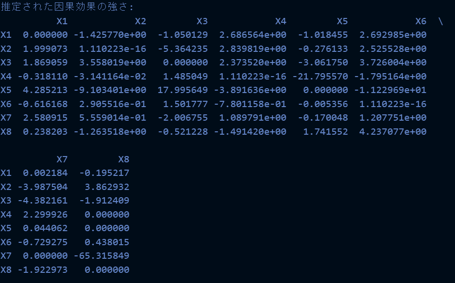ロジスティック回帰祭りの時よりも結果的には、良さそうな感じもしなくもないですね。サンプルデータが完全に線形で規定されているからというのもありますが...実際のデータだとどうなんでしょうね？

非線形拡張版のLiNGAM

非線形拡張版のLiNGAM（以下、非線形LiNGAM）は、従来のLiNGAMモデルを拡張し、変数間の非線形な関係性を扱えるようにした手法です。この拡張により、より複雑で現実的な因果関係のモデリングが可能になりました。
非線形LiNGAMの基本モデルは以下の数式で表現されます

$x_j = f_j(pa_j) + e_j$

ここで

$x_j$ は $j$ 番目の観測変数

$f_j$ は非線形関数

$pa_j$ は $x_j$ の親変数（直接の原因となる変数）の集合

$e_j$ は外生変数（ノイズ項）

　　
この式は、各変数が親変数の非線形関数とノイズ項の和で表現されることを示しています。従来のLiNGAMと同様に、因果関係に循環がないことを仮定しています。

非線形LiNGAMの重要な特徴は、非線形関数 $f_j$ をどのようにモデル化するかにあります。一般的なアプローチとしては、加法モデルを使用する方法があります

$f_j(pa_j) = \sum_{k \in pa_j} f_{jk}(x_k)$

ここで、 $f_{jk}$ は $x_k$ から $x_j$ への非線形効果を表す関数です。これらの関数は、スプライン関数やカーネル法など、様々な非線形回帰手法を用いてモデル化されます。

　　
非線形LiNGAMの推定プロセスは、以下のステップで行われます
1. 非線形独立成分分析（非線形ICA）を用いて、データを互いに独立な非線形成分に分解します。
2. 得られた独立成分間の依存関係を評価し、因果順序を推定します。
3. 推定された因果順序に基づいて、各変数の非線形モデルを構築します。
　　
このプロセスでは、非線形ICAが重要な役割を果たします。非線形ICAは以下の式で表現されます

$x = f(s)$

ここで

$f$ は非線形混合関数

$s$ は互いに独立な非ガウス信号源

　　
非線形LiNGAMの理論的背景には、非線形性と非ガウス性を組み合わせることで、より複雑な因果構造を識別できるという洞察があります。非線形性を導入することで、変数間の複雑な相互作用をモデル化できるようになり、より現実的なシステムの分析が可能になります。
しかし、非線形LiNGAMにも課題があります。非線形モデルの推定は線形モデルよりも複雑で、計算コストが高くなります。また、モデルの複雑さが増すことで、過学習のリスクも高まります。さらに、非線形関数の選択や、モデルの解釈可能性の確保なども重要な課題となります。
これらの課題に対処するため、様々な手法が提案されています。例えば、スパース性を導入することで過学習を抑制したり、解釈可能な非線形関数を使用したりする方法があります。また、ベイズ推論を用いてモデルの不確実性を評価する手法も開発されています。

非線形拡張のLiNGAM実装してみた

import numpy as np
import pandas as pd
from sklearn.preprocessing import StandardScaler
from sklearn.kernel_approximation import RBFSampler
import pydot
import colorsys
from scipy import stats
from sklearn.gaussian_process.kernels import RBF
from scipy.optimize import minimize

class NonlinearLiNGAM:
    def __init__(self, n_components=None, gamma='scale'):
        # 因果順序と隣接行列を保持するための変数を初期化
        self.causal_order_ = None
        self.adjacency_matrix_ = None
        self.n_components = n_components
        self.gamma = gamma

    def fit(self, X):
        # DataFrameの場合はnumpy配列に変換
        if isinstance(X, pd.DataFrame):
            X = X.values
        n, p = X.shape
        
        # n_componentsが指定されていない場合、元のデータの次元数を使用
        if self.n_components is None:
            self.n_components = p

        # RBFSamplerの初期化
        self.rbf_sampler = RBFSampler(n_components=self.n_components, gamma=self.gamma)
        
        # Step 1: データの非線形変換
        X_nonlinear = self.rbf_sampler.fit_transform(X)

        # Step 2: 非線形ICAの適用
        W = self._nonlinear_ica(X_nonlinear)

        # Step 3: 因果順序の推定
        causal_order = self._estimate_causal_order(W)

        # Step 4: 非線形因果効果の推定
        B = np.zeros((p, p))
        for i, idx in enumerate(causal_order):
            parents = causal_order[:i]
            if len(parents) > 0:
                effect = self._estimate_nonlinear_effect(X[:, parents], X[:, idx])
                B[parents, idx] = effect.ravel()[:len(parents)]

        # Step 5: プルーニング
        B = self._pruning(X, B)

        # 推定された因果順序と隣接行列を保存
        self.causal_order_ = causal_order
        self.adjacency_matrix_ = B
        return self

    def _nonlinear_ica(self, X, max_iter=1000, tol=1e-4):
        """非線形ICAの実装"""
        n, p = X.shape
        # ランダムな初期の重み行列を生成
        W = np.random.randn(p, p)
        for iteration in range(max_iter):
            W_new = self._ica_iteration(X, W)
            # 収束判定
            if np.max(np.abs(np.abs(np.diag(np.dot(W_new, W.T))) - 1)) < tol:
                break
            W = W_new
        return W

    def _ica_iteration(self, X, W):
        """ICAの1イテレーション"""
        Z = np.dot(W, X.T)
        G = np.tanh(Z)  # 非線形関数（ここではtanh）を適用
        G_der = 1 - G**2  # 非線形関数の導関数
        W_new = np.dot(G, X) / X.shape[0] - np.diag(G_der.mean(axis=1)) @ W
        return self._symmetric_decorrelation(W_new)

    def _symmetric_decorrelation(self, W):
        """対称直交化"""
        U, S, Vt = np.linalg.svd(W)
        return np.dot(U, Vt)

    def _estimate_causal_order(self, W):
        """因果順序の推定"""
        p = W.shape[0]
        causal_order = list(range(p))
        for i in range(p-1):
            for j in range(i+1, p):
                if np.abs(W[causal_order[i], causal_order[j]]) < np.abs(W[causal_order[j], causal_order[i]]):
                    causal_order[i], causal_order[j] = causal_order[j], causal_order[i]
        return causal_order

    def _estimate_nonlinear_effect(self, X, y):
        """非線形因果効果の推定"""
        def objective(theta):
            kernel = RBF(length_scale=theta[0])
            K = kernel(X)
            return np.mean((y - K @ np.linalg.inv(K + 1e-8 * np.eye(K.shape[0])) @ y) ** 2)
        
        res = minimize(objective, x0=[1.0], method='L-BFGS-B', bounds=[(1e-5, None)])
        kernel = RBF(length_scale=res.x[0])
        K = kernel(X)
        return np.linalg.inv(K + 1e-8 * np.eye(K.shape[0])) @ y.reshape(-1, 1)

    def _pruning(self, X, B, alpha=0.05):
        """
        推定された因果構造のプルーニング
        統計的に有意でない因果関係を除去する
        """
        n, p = X.shape
        for i in range(p):
            parents = np.where(B[:, i] != 0)[0]
            if len(parents) > 0:
                X_parents = X[:, parents]
                residual = X[:, i] - X_parents @ B[parents, i]
                for j in parents:
                    X_j = X[:, j]
                    # スピアマンの順位相関係数を計算（非線形関係に対応）
                    r, p_value = stats.spearmanr(X_j, residual)
                    # 有意でない場合、因果関係を除去
                    if p_value > alpha:
                        B[j, i] = 0
        return B

    def plot_dag(self, column_names, output_file='nonlinear_lingam_dag.png', threshold=0.1):
        """因果構造をDAGとして描画"""
        graph = pydot.Dot(graph_type='digraph', rankdir='LR')
        
        # ノードの追加
        nodes = {}
        for col in column_names:
            node = pydot.Node(col, style="filled", fillcolor="lightblue")
            graph.add_node(node)
            nodes[col] = node
        
        # エッジの追加
        max_effect = np.max(np.abs(self.adjacency_matrix_))
        for i, from_var in enumerate(column_names):
            for j, to_var in enumerate(column_names):
                effect = self.adjacency_matrix_[i, j]
                if i != j and np.abs(effect) > threshold:
                    # 効果の強さに基づいて線の太さを決定（1〜5の範囲）
                    penwidth = 1 + 4 * (np.abs(effect) / max_effect)
                    
                    # 効果の強さと符号に基づいて色を決定
                    if effect > 0:
                        hue = 0.33  # 緑色
                    else:
                        hue = 0  # 赤色
                    saturation = 0.5 + 0.5 * (np.abs(effect) / max_effect)
                    rgb = colorsys.hsv_to_rgb(hue, saturation, 1)
                    color = '#{:02x}{:02x}{:02x}'.format(int(rgb[0]*255), int(rgb[1]*255), int(rgb[2]*255))
                    
                    # エッジを追加
                    edge = pydot.Edge(nodes[from_var], nodes[to_var], 
                                      label=f"{effect:.2f}", 
                                      penwidth=penwidth, 
                                      color=color)
                    graph.add_edge(edge)
        
        # PNG画像として保存
        graph.write_png(output_file)
        
        return output_file

実行してみたコードは以下です。私の環境では2分くらいかかりました。

import numpy as np
import pandas as pd
from sklearn.preprocessing import StandardScaler
from sklearn.kernel_approximation import RBFSampler
import pydot
import colorsys
from scipy import stats
from sklearn.gaussian_process.kernels import RBF
from scipy.optimize import minimize

# サンプルデータの生成（非線形関係を含む）
np.random.seed(42)
n_samples = 2000

# 各変数の生成（非線形関係を含む）
x1 = np.random.binomial(1, 0.6, n_samples)
x2 = 2 * np.sin(x1) + np.random.normal(0, 1, n_samples)
x3 = 1.5 * x1 + 0.8 * x2**2 + np.random.normal(0, 1, n_samples)
x4 = np.random.binomial(1, 0.4, n_samples)
x5 = 2.5 * np.exp(x4) + np.random.normal(0, 1, n_samples)
x6 = 1.2 * np.tanh(x3) + 0.9 * x5 + np.random.normal(0, 1, n_samples)
x7 = np.random.binomial(1, 1 / (1 + np.exp(-(0.8 * x2 + 0.6 * x6))), n_samples)
x8 = 0.3 * np.sin(x1) + 0.2 * x2**2 + 0.2 * np.exp(x3) + 0.3 * x4 + 0.2 * np.log(np.abs(x5) + 1) + 0.2 * x6 + 0.3 * x7 + np.random.normal(0, 1, n_samples)

# DataFrameの作成
df = pd.DataFrame({
    'X1': x1, 'X2': x2, 'X3': x3, 'X4': x4,
    'X5': x5, 'X6': x6, 'X7': x7, 'X8': x8
})

# データの標準化
scaler = StandardScaler()
df_scaled = pd.DataFrame(scaler.fit_transform(df), columns=df.columns)

# 非線形LiNGAMの適用とDAGの描画
model = NonlinearLiNGAM()
model.fit(df_scaled)
output_file = model.plot_dag(df_scaled.columns, output_file='nonlinear_lingam_dag.png')

# 推定された因果効果の強さを表示
print("\n推定された因果効果の強さ:")
print(pd.DataFrame(model.adjacency_matrix_, columns=df.columns, index=df.columns))

実行結果は以下です。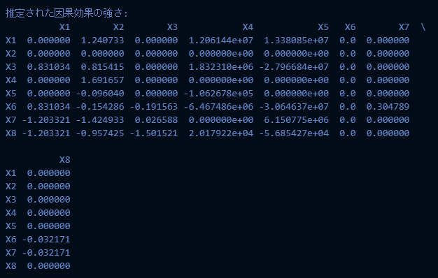今回の非線形LiNGAMの実装は以下です。
1. RBFSamplerを使用して、入力データを高次元の特徴空間に変換します。これによって非線形関係をとらえる感じです。
2. 非線形ICAを適用して、独立成分を見つけます
3. 非線形因果効果の推定には、ガウス過程回帰を使用します。これにより、変数間の非線形関係をモデル化します。
4. プルーニングでは、スピアマンの順位相関係数を使用します。これは非線形関係にも適用可能です。
5. DAGの描画方法は線形LiNGAMと同じですが、エッジの重みは非線形効果を表しています。
　　
非線形LiNGAMは実行時間が長いのと、解釈がどう解釈したらいいのかが難しいですね... あまり使う機会はなさそうな感じが個人的にはしますね

非線形LiNGAM（ベイズで実装）

実装のコードは以下です。

class BayesianNonlinearLiNGAM:
    def __init__(self, n_components=30, gamma='scale', n_iter=2000, n_warmup=1000):
        self.causal_order_ = None
        self.adjacency_matrix_ = None
        self.adjacency_matrix_std_ = None
        self.n_components = n_components
        self.gamma = gamma
        self.n_iter = n_iter
        self.n_warmup = n_warmup

    def fit(self, X):
        if isinstance(X, pd.DataFrame):
            X = X.values
        n, p = X.shape
        
        self.rbf_samplers = [RBFSampler(n_components=self.n_components, gamma=self.gamma, random_state=42) for _ in range(p)]
        X_nonlinear = np.hstack([sampler.fit_transform(X[:, [i]]) for i, sampler in enumerate(self.rbf_samplers)])
        
        ica = FastICA(n_components=p, random_state=42, whiten='unit-variance')
        S = ica.fit_transform(X_nonlinear)
        W = ica.mixing_

        causal_order = self._estimate_causal_order(W)

        B = np.zeros((p, p))
        B_std = np.zeros((p, p))
        for i in range(p):
            parents = causal_order[:i]
            if len(parents) > 0:
                effects, stds = self._bayesian_nonlinear_regression(X[:, parents], X[:, i])
                B[parents, i] = effects
                B_std[parents, i] = stds

        B, B_std = self._bayesian_pruning(X, B, B_std, threshold=0.05)

        self.causal_order_ = causal_order
        self.adjacency_matrix_ = B
        self.adjacency_matrix_std_ = B_std
        return self

    def _estimate_causal_order(self, W):
        p = W.shape[1]
        causal_order = list(range(p))
        for i in range(p-1):
            for j in range(i+1, p):
                if np.abs(W[:, causal_order[i]]).mean() < np.abs(W[:, causal_order[j]]).mean():
                    causal_order[i], causal_order[j] = causal_order[j], causal_order[i]
        return causal_order

    def _bayesian_nonlinear_regression(self, X, y):
        X_nonlinear = np.hstack([sampler.transform(X[:, [i]]) for i, sampler in enumerate(self.rbf_samplers[:X.shape[1]])])
        n, p = X_nonlinear.shape

        # Stanモデルの定義
        stan_code = f"""
        data {{
          int<lower=0> N;
          int<lower=0> P;
          matrix[N, P] X;
          vector[N] y;
        }}
        parameters {{
          vector[P] beta;
          real<lower=0> sigma;
        }}
        model {{
          beta ~ normal(0, 10);
          sigma ~ inv_gamma(2, 0.1);
          y ~ normal(X * beta, sigma);
        }}
        """

        # 一時ファイルにStanコードを書き込む
        with tempfile.NamedTemporaryFile(mode='w', suffix='.stan', delete=False) as temp_file:
            temp_file.write(stan_code)
            temp_file_name = temp_file.name

        # Stanモデルのコンパイルと実行
        model = CmdStanModel(stan_file=temp_file_name)
        data = {'N': n, 'P': p, 'X': X_nonlinear, 'y': y}
        fit = model.sample(data=data, iter_sampling=self.n_iter, iter_warmup=self.n_warmup, chains=12)

        # 一時ファイルの削除
        import os
        os.unlink(temp_file_name)

        # 結果の抽出
        az_data = az.from_cmdstanpy(posterior=fit)
        summary = az.summary(az_data)
        effects = summary['mean'].values[:-1]  # sigmaを除外
        stds = summary['sd'].values[:-1]  # sigmaを除外

        return effects[:len(X[0])], stds[:len(X[0])]  # parentsの長さに合わせる

    def _bayesian_pruning(self, X, B, B_std, threshold=0.05):
        n, p = X.shape
        for i in range(p):
            parents = np.where(B[:, i] != 0)[0]
            if len(parents) > 0:
                for j in parents:
                    if np.abs(B[j, i]) < threshold * B_std[j, i]:
                        B[j, i] = 0
                        B_std[j, i] = 0
        return B, B_std

    def plot_dag(self, column_names, output_file='bayesian_nonlinear_lingam_dag.png', threshold=0.01):
        graph = pydot.Dot(graph_type='digraph', rankdir='LR')
        
        # ノードの追加
        nodes = {}
        for col in column_names:
            node = pydot.Node(col, style="filled", fillcolor="lightblue")
            graph.add_node(node)
            nodes[col] = node
        
        # エッジの追加
        max_effect = np.max(np.abs(self.adjacency_matrix_))
        for i, from_var in enumerate(column_names):
            for j, to_var in enumerate(column_names):
                effect = self.adjacency_matrix_[i, j]
                std = self.adjacency_matrix_std_[i, j]
                if i != j and np.abs(effect) > threshold:
                    # 効果の強さに基づいて線の太さを決定
                    penwidth = 1 + 4 * (np.abs(effect) / max_effect)
                    
                    # 効果の符号に基づいて色を決定
                    if effect > 0:
                        hue = 0.33  # 緑色
                    else:
                        hue = 0  # 赤色
                    saturation = 0.5 + 0.5 * (np.abs(effect) / max_effect)
                    rgb = colorsys.hsv_to_rgb(hue, saturation, 1)
                    color = '#{:02x}{:02x}{:02x}'.format(int(rgb[0]*255), int(rgb[1]*255), int(rgb[2]*255))
                    
                    # エッジを追加
                    edge = pydot.Edge(nodes[from_var], nodes[to_var], 
                                      label=f"{effect:.2f}±{std:.2f}", 
                                      penwidth=penwidth, 
                                      color=color)
                    graph.add_edge(edge)
        
        # PNG画像として保存
        graph.write_png(output_file)
        
        return output_file

以下が実行してみたのコードです

import numpy as np
import pandas as pd
from sklearn.preprocessing import StandardScaler
from sklearn.kernel_approximation import RBFSampler
from sklearn.decomposition import FastICA
import pydot
import colorsys
from cmdstanpy import CmdStanModel
import arviz as az
import tempfile

np.random.seed(42)
n_samples = 2000

x1 = np.random.binomial(1, 0.6, n_samples)
x2 = 2 * np.sin(x1) + np.random.normal(0, 1, n_samples)
x3 = 1.5 * x1 + 0.8 * x2**2 + np.random.normal(0, 1, n_samples)
x4 = np.random.binomial(1, 0.4, n_samples)
x5 = 2.5 * np.exp(x4) + np.random.normal(0, 1, n_samples)
x6 = 1.2 * np.tanh(x3) + 0.9 * x5 + np.random.normal(0, 1, n_samples)
x7 = np.random.binomial(1, 1 / (1 + np.exp(-(0.8 * x2 + 0.6 * x6))), n_samples)
x8 = 0.3 * np.sin(x1) + 0.2 * x2**2 + 0.2 * np.exp(x3) + 0.3 * x4 + 0.2 * np.log(np.abs(x5) + 1) + 0.2 * x6 + 0.3 * x7 + np.random.normal(0, 1, n_samples)

df = pd.DataFrame({
    'X1': x1, 'X2': x2, 'X3': x3, 'X4': x4,
    'X5': x5, 'X6': x6, 'X7': x7, 'X8': x8
})

scaler = StandardScaler()
df_scaled = pd.DataFrame(scaler.fit_transform(df), columns=df.columns)

model = BayesianNonlinearLiNGAM()
model.fit(df_scaled)

output_file = model.plot_dag(df_scaled.columns, output_file='bayesian_nonlinear_lingam_dag.png')
print(f"ベイズ非線形LiNGAMのDAGが {output_file} として保存されました。")

print("\n推定された因果効果の強さ（平均±標準偏差）:")
for i, row in enumerate(model.adjacency_matrix_):
     for j, val in enumerate(row):
        if i != j and val != 0:
            print(f"{df.columns[i]} -> {df.columns[j]}: {val:.3f}±{model.adjacency_matrix_std_[i,j]:.3f}")

print("\n隣接行列:")
print(model.adjacency_matrix_)

今回はベイズの部分でcmdstanpyを使用しています。今回の件から外れますが、cmdstanpyをインストールするときは、conda installを使いましょう。pipはまじでめんどくさいです。WindowsだとRToolsをインストールしなくてはならず、そのうえPATHの設定も必要で、それでもmakeというものが原因で私の環境ではエラー吐いて動きませんでした。
conda installなら、インストールした後に、import cmdstanpy, cmdstanpy.install_cmdstan()でTrueとなれば環境構築が終わります。断然conda installがおすすめです。
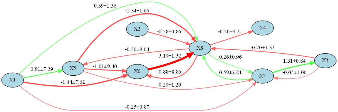
実行結果は以下です。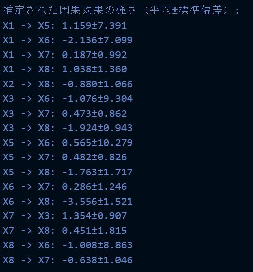因みに、実行に2時間かかりました。（高性能なPCが欲しい...）実務では実行時間長くて使いづらそうですね、ただ推定結果は結構信頼できそうな結果が得られた感じします。ただのLiNGAMで把握して、変数を絞って非線形ベイズLiNGAMで因果探索くらいはありかもしれませんが...
後段の時系列用のLiNGAMではベイズ版の実装もしようかと思ったのですが、さすがにもう疲れたので、単純なもので許してください。

TimeSeriesLiNGAM（時系列LiNGAM）

TimeSeriesLiNGAM（時系列LiNGAM）は、従来のLiNGAMを時系列データに適用できるように拡張したモデルです。この手法は、時間的な依存関係を持つデータにおける因果構造を推定することを目的としています。
TimeSeriesLiNGAMの基本モデルは以下の数式で表現されます

$x(t) = \sum_{k=0}^K B_k x(t-k) + e(t)$

ここで

$x(t)$ は時刻 $t$ における観測変数のベクトル

$B_k$ は $k$ 時点前の変数が現在の変数に与える影響を表す係数行列

$K$ は考慮する最大のラグ

$e(t)$ は外生変数（ノイズ項）のベクトル

この式は、各時点の変数が過去の変数の線形結合とノイズ項の和で表現されることを示しています。 $B_0$ は同時点での因果効果を表し、LiNGAMと同様に下三角行列（または行列の並べ替えで下三角になる行列）であることが仮定されます。

TimeSeriesLiNGAMの重要な特徴は、時間的な因果関係と同時点での因果関係を同時にモデル化できる点です。これにより、複雑な動的システムにおける因果構造をより正確に推定することが可能になります。
モデルの推定プロセスは以下のステップで行われます
1. 自己回帰（AR）モデルを用いて、各変数の時系列的な依存関係を除去します。
2. 残差に対して通常のLiNGAMを適用し、同時点での因果構造を推定します。
3. 推定された因果順序に基づいて、時間的な因果効果と同時点での因果効果を再推定します。
　　
このプロセスを数式で表現すると以下のようになります
まず、ARモデルを適用します

$x(t) = \sum_{k=1}^K A_k x(t-k) + r(t)$

ここで、 $A_k$ はARモデルの係数行列、 $r(t)$ は残差です。

次に、残差 $r(t)$ に対してLiNGAMを適用します

$r(t) = B_0 r(t) + e(t)$

ここで、 $B_0$ は同時点での因果効果を表す行列です。

　　
最後に、元のモデルのパラメータを再構成します

$B_0 = I - (I - B_0)^{-1}$

$B_k = (I - B_0)^{-1} A_k$ for $k>0$

TimeSeriesLiNGAMの理論的背景には、時系列データにおける因果の概念を明確化し、グレンジャー因果性とLiNGAMの考え方を統合するという洞察があります。この手法により、時間的な先行関係だけでなく、同時点での因果関係も考慮した包括的な因果モデルを構築することが可能になります。

しかし、TimeSeriesLiNGAMにも課題があります。例えば、適切なラグ次数 $K$ の選択や、非定常性への対処、長期的な因果関係の捕捉などが挙げられます。また、時系列データの特性（季節性、トレンドなど）によっては、前処理や追加的なモデリングが必要になる場合があります。

TimeSeriesLiNGAMを実装してみた（線形のです）

import numpy as np
import pandas as pd
from scipy import stats
import pydot
import colorsys
from sklearn.preprocessing import StandardScaler
from statsmodels.tsa.ar_model import AutoReg

class TimeSeriesLiNGAM:
    def __init__(self, lags=1):
        self.lags = lags
        self.causal_order_ = None
        self.adjacency_matrices_ = None
        self.ar_coefficients_ = None

    def fit(self, X):
        if isinstance(X, pd.DataFrame):
            X = X.values
        
        n, p = X.shape
        
        residuals = self._apply_ar_model(X)
        lingam_model = self._apply_lingam(residuals)
        
        self.causal_order_ = lingam_model.causal_order_
        B = lingam_model.adjacency_matrix_
        
        self._reestimate_effects(X, B)
        
        return self

    def _apply_ar_model(self, X):
        n, p = X.shape
        residuals_list = []
        self.ar_coefficients_ = []
        
        for i in range(p):
            model = AutoReg(X[:, i], lags=self.lags, old_names=False)
            results = model.fit()
            self.ar_coefficients_.append(results.params)
            residuals_list.append(results.resid[self.lags:])
        
        min_length = min(len(res) for res in residuals_list)
        residuals = np.column_stack([res[:min_length] for res in residuals_list])
        
        return residuals

    def _apply_lingam(self, residuals):
        lingam_model = LiNGAM()
        lingam_model.fit(residuals)
        return lingam_model

    def _reestimate_effects(self, X, B):
        n, p = X.shape
        self.adjacency_matrices_ = [np.zeros((p, p)) for _ in range(self.lags + 1)]
        
        X_lagged = []
        for lag in range(self.lags + 1):
            X_lagged.append(X[self.lags - lag : -lag if lag > 0 else None])
        X_lagged = np.hstack(X_lagged)
        
        for i, idx in enumerate(self.causal_order_):
            y = X_lagged[:, idx]
            X_parents = np.zeros((len(y), 0))
            
            simultaneous_parents = [self.causal_order_[j] for j in range(i) if B[self.causal_order_[j], idx] != 0]
            if simultaneous_parents:
                X_parents = np.column_stack((X_parents, X_lagged[:, simultaneous_parents]))
            
            X_parents = np.column_stack((X_parents, X_lagged[:, p:]))
            
            coeffs = np.linalg.lstsq(X_parents, y, rcond=None)[0]
            
            coeff_idx = 0
            if simultaneous_parents:
                self.adjacency_matrices_[0][idx, simultaneous_parents] = coeffs[:len(simultaneous_parents)]
                coeff_idx = len(simultaneous_parents)
            
            for lag in range(1, self.lags + 1):
                self.adjacency_matrices_[lag][:, idx] = coeffs[coeff_idx:coeff_idx+p]
                coeff_idx += p

    def plot_dag(self, column_names, output_file='timeseries_lingam_dag.png', threshold=0.01):
        graph = pydot.Dot(graph_type='digraph', rankdir='TB')
        
        nodes = {}
        for t in range(self.lags, -1, -1):
            for col in column_names:
                node_name = f"{col}_t-{t}"
                fillcolor = "lightblue" if t == 0 else "white"
                node = pydot.Node(node_name, style="filled", fillcolor=fillcolor)
                graph.add_node(node)
                nodes[node_name] = node
        
        max_effect = max(np.max(np.abs(adj_mat)) for adj_mat in self.adjacency_matrices_)
        
        for i, from_idx in enumerate(self.causal_order_):
            from_var = column_names[from_idx]
            for j in range(i+1, len(self.causal_order_)):
                to_idx = self.causal_order_[j]
                to_var = column_names[to_idx]
                effect = self.adjacency_matrices_[0][to_idx, from_idx]
                if np.abs(effect) > threshold:
                    self._add_edge(graph, nodes, f"{from_var}_t-0", f"{to_var}_t-0", effect, max_effect)
        
        for t in range(1, self.lags + 1):
            for from_idx, from_var in enumerate(column_names):
                for to_idx, to_var in enumerate(column_names):
                    effect = self.adjacency_matrices_[t][to_idx, from_idx]
                    if np.abs(effect) > threshold:
                        self._add_edge(graph, nodes, f"{from_var}_t-{t}", f"{to_var}_t-0", effect, max_effect)
        
        graph.write_png(output_file)
        return output_file

    def _add_edge(self, graph, nodes, from_node, to_node, effect, max_effect):
        penwidth = 1 + 4 * (np.abs(effect) / max_effect)
        hue = 0.33 if effect > 0 else 0
        saturation = 0.5 + 0.5 * (np.abs(effect) / max_effect)
        rgb = colorsys.hsv_to_rgb(hue, saturation, 1)
        color = '#{:02x}{:02x}{:02x}'.format(int(rgb[0]*255), int(rgb[1]*255), int(rgb[2]*255))
        edge = pydot.Edge(nodes[from_node], nodes[to_node], 
                        label=f"{effect:.2f}", 
                        penwidth=penwidth, 
                        color=color)
        graph.add_edge(edge)

    def preprocess_data(self, X):
        if isinstance(X, pd.DataFrame):
            X = X.values
        
        n, p = X.shape
        X_processed = np.zeros_like(X)
        
        for i in range(p):
            if len(np.unique(X[:, i])) == 2:
                X_processed[:, i] = X[:, i]
            else:
                scaler = StandardScaler()
                X_processed[:, i] = scaler.fit_transform(X[:, i].reshape(-1, 1)).flatten()
        
        return X_processed

    def fit_preprocess(self, X):
        X_processed = self.preprocess_data(X)
        return self.fit(X_processed)

class LiNGAM:
    def __init__(self):
        self.causal_order_ = None
        self.adjacency_matrix_ = None

    def fit(self, X):
        n, p = X.shape
        
        X_centered = X - X.mean(axis=0)
        cov = np.cov(X_centered, rowvar=False)
        eig_vals, eig_vecs = np.linalg.eigh(cov)
        W = np.dot(np.diag(1.0 / np.sqrt(eig_vals)), eig_vecs.T)
        X_white = np.dot(X_centered, W.T)

        W_ = self._fastICA(X_white)
        B = np.dot(W_, W)

        self.causal_order_ = self._estimate_causal_order(B)
        B_perm = B[self.causal_order_][:, self.causal_order_]

        D = np.diag(1.0 / np.diag(B_perm))
        self.adjacency_matrix_ = np.eye(p) - np.dot(D, B_perm)
        
        return self

    def _fastICA(self, X, max_iter=1000, tol=1e-4):
        n, p = X.shape
        W = np.random.randn(p, p)
        for iteration in range(max_iter):
            W_new = self._ica_iteration(X, W)
            if np.max(np.abs(np.abs(np.diag(np.dot(W_new, W.T))) - 1)) < tol:
                break
            W = W_new
        return W

    def _ica_iteration(self, X, W):
        Z = np.dot(W, X.T)
        G = np.tanh(Z)
        G_der = 1 - G**2
        W_new = np.dot(G, X) / X.shape[0] - np.diag(G_der.mean(axis=1)) @ W
        return self._symmetric_decorrelation(W_new)

    def _symmetric_decorrelation(self, W):
        U, S, Vt = np.linalg.svd(W)
        return np.dot(U, Vt)

    def _estimate_causal_order(self, B):
        p = B.shape[0]
        causal_order = list(range(p))
        for i in range(p-1):
            for j in range(i+1, p):
                if np.abs(B[causal_order[i], causal_order[j]]) < np.abs(B[causal_order[j], causal_order[i]]):
                    causal_order[i], causal_order[j] = causal_order[j], causal_order[i]
        return causal_order

実行例は以下です

import numpy as np
import pandas as pd
from scipy import stats
import pydot
import colorsys
from sklearn.preprocessing import StandardScaler
from statsmodels.tsa.ar_model import AutoReg

# サンプルデータの生成
np.random.seed(0)
n = 1000
x1 = np.random.randn(n)
x2 = 0.5 * x1 + np.random.randn(n)
x3 = 0.3 * x1 + 0.5 * x2 + np.random.randn(n)
binary = np.random.binomial(1, 0.5, n)

data = pd.DataFrame({
    'x1': x1,
    'x2': x2,
    'x3': x3,
    'binary': binary
})

# モデルの適用
model = TimeSeriesLiNGAM(lags=2)
model.fit_preprocess(data)

# DAGの描画
model.plot_dag(data.columns, 'timeseries_lingam_dag.png')

実行結果は以下です。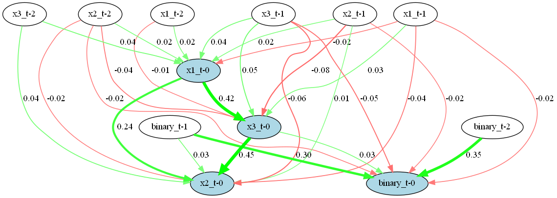このTimeSeriesLiNGAMクラスの実装内容は基本的に理論の解説と同様です。

最後に

私も大変興味がある手法だったので、実装含め結構重めに扱ってみました。非線形でベイズでやる方法を実装してみようとしたところ、めちゃくちゃ大変で、実装するのにめちゃくちゃ苦労しました。実務で使える機会を見つけたら、この労力が無駄じゃなかったことを証明するために、非線形ベイズLiNGAMは使おうと思っています。使ってあげないとむしろかわいそうです。あと通常のLiNGAMライブラリでDAGの描画ってできないんですかね？
私が何かミスってただけなんですかね？おかげでフルスクラッチで実装する羽目になり、理解は進みましたが、使えるなら既存のツールを使いたいものですよね... 以前のロジスティック回帰祭りのなんちゃって因果探索よりは、理論的に裏付けのある手法なので、こっちの方がいいんですかね？
私も因果探索にあまり詳しくなく、最近勉強してる感じなので、どれがいいのかは手探り状態という感じですね。
なにかいい情報があれば、コメントででも教えてくださると助かります。ここまで読んでくださりありがとうございました。