はじめに
今回は前回までの、機械学習モデルの理論の解説とは異なり、私が最も関心のある、因果推論の分野に関しての内容に入っていきたいと思います。これらの手法はCATE(条件付き平均処置効果)というものを推定するものです。
Causal Tree
Causal Treeは、従来の決定木アルゴリズムを拡張し、因果推論の文脈に適用したものです。この手法の主な目的は、異質性のある処置効果を捉え、個々のサブグループに対する条件付き平均処置効果(CATE)を推定することです。
CATE(条件付き平均処置効果)
CATE(Conditional Average Treatment Effect)は、特定の共変量の値に条件付けられた平均処置効果を指します。より形式的には、以下のように定義されます:
ここで
CATEは、潜在的結果フレームワーク(Potential Outcomes Framework)に基づいています。このフレームワークでは、各個体に対して処置を受けた場合と受けなかった場合の両方の結果が存在すると仮定します。しかし、現実世界では、我々は各個体に対してどちらか一方の結果しか観察することができません。これは基本的な因果推論の問題であり、「基本的な問題」(Fundamental Problem of Causal Inference)と呼ばれています。
CATEは、この問題に対処するために、特定の共変量の値を持つ個体群に対する平均的な処置効果を推定しようとします。つまり、似た特徴を持つ個体群の中で、処置を受けた場合と受けなかった場合の結果の期待値の差を計算します。
CATEの推定には以下のような重要な仮定が必要です
CATEの推定は、異質性のある処置効果を理解する上で非常に重要です。例えば、ある治療法が平均的には効果があるとしても、特定のサブグループ(例:高齢者や特定の遺伝子を持つ人)では効果が異なる可能性があります。CATEを推定することで、このような異質性を捉え、より精密な治療法の選択や政策の立案が可能になります。
Causal TreeやCausal Forestなどの手法は、このCATEを非パラメトリックに推定するための方法です。これらの手法は、データ駆動型のアプローチで共変量空間を分割し、各領域でのCATEを推定します。これにより、処置効果の複雑な非線形性や交互作用を柔軟にモデル化することができます。
CATEを用いてATEを推定する
また、別の話として、CATEを用いて全体の平均処置効果(ATE)を推定することもできます。まず、ATEの定義は以下のようです。
CATEで特定のサブグループに対する処置効果の推定
これ以外にも、特定のサブグループに対する処置効果の推定も可能です。
また、この話から分かるように、ATTやATUの推定も可能になります。
ATTは、実際に処置を受けた個体に対する平均処置効果を表します。
個別処置効果(ITE: Individual Treatment Effect)の推定
ここまでの説明で、CATE自体が正しく推定できていれば、様々な効果検証が可能ということはご理解いただけたかなと思います。
目的関数
この目的関数は、実際の結果と推定された処置効果との差の二乗和を最小化しようとしています。ここでの重要な点は、通常の決定木が予測値自体を最適化するのに対し、Causal Treeは処置効果の推定値を最適化しようとしていることです。これにより、処置効果の異質性を直接モデル化することが可能になります。
CATE推定の詳細
この式は、各葉ノードにおけるCATEの推定方法を示しています。本質的には、処置群と対照群の結果の平均差を計算しています。この方法は、潜在的結果フレームワーク(Potential Outcomes Framework)に基づいており、各個体が処置を受けた場合と受けなかった場合の結果の差を推定しようとしています。
ここで重要なのは、この推定が各葉ノード内で行われることです。つまり、特定の特徴を持つサブグループ(葉ノードで表現される)ごとに処置効果を推定することができ、これにより処置効果の異質性を捉えることができます。
分割基準
Causal Treeの分割プロセスは、処置効果の異質性を最大化することを目指します。具体的には、以下のステップで行われます
Causal Treeのフルスクラッチ実装
import numpy as np
from typing import List, Tuple, Optional

class CausalTreeNode:
    def __init__(self, depth: int = 0):
        self.feature_index: Optional[int] = None
        self.threshold: Optional[float] = None
        self.tau: Optional[float] = None
        self.left: Optional[CausalTreeNode] = None
        self.right: Optional[CausalTreeNode] = None
        self.depth: int = depth

class CausalTree:
    def __init__(self, max_depth: int = 5, min_samples_leaf: int = 10):
        self.root: Optional[CausalTreeNode] = None
        self.max_depth: int = max_depth
        self.min_samples_leaf: int = min_samples_leaf

    def fit(self, X: np.ndarray, y: np.ndarray, w: np.ndarray):
        """
        モデルを学習する
        X: 特徴量, y: 結果変数, w: 処置変数
        """
        self.root = self._build_tree(X, y, w)

    def _build_tree(self, X: np.ndarray, y: np.ndarray, w: np.ndarray, depth: int = 0) -> CausalTreeNode:
        node = CausalTreeNode(depth)

        # 葉ノードの条件をチェック
        if depth == self.max_depth or len(y) <= self.min_samples_leaf:
            node.tau = self._estimate_tau(y, w)
            return node

        # 最適な分割を見つける
        best_feature, best_threshold = self._find_best_split(X, y, w)

        if best_feature is None:
            # これ以上分割できない場合
            node.tau = self._estimate_tau(y, w)
            return node

        # ノードの情報を設定
        node.feature_index = best_feature
        node.threshold = best_threshold

        # データを分割
        left_mask = X[:, best_feature] <= best_threshold
        right_mask = ~left_mask

        # 子ノードを再帰的に構築
        node.left = self._build_tree(X[left_mask], y[left_mask], w[left_mask], depth + 1)
        node.right = self._build_tree(X[right_mask], y[right_mask], w[right_mask], depth + 1)

        return node

    def _find_best_split(self, X: np.ndarray, y: np.ndarray, w: np.ndarray) -> Tuple[Optional[int], Optional[float]]:
        """
        最適な分割を見つける
        """
        best_feature = None
        best_threshold = None
        best_mse_reduction = 0

        n_features = X.shape[1]

        for feature in range(n_features):
            thresholds = np.unique(X[:, feature])
            for threshold in thresholds:
                left_mask = X[:, feature] <= threshold
                right_mask = ~left_mask

                # 各子ノードのサンプル数が最小サンプル数以上であることを確認
                if np.sum(left_mask) < self.min_samples_leaf or np.sum(right_mask) < self.min_samples_leaf:
                    continue

                mse_reduction = self._calculate_mse_reduction(y, w, left_mask, right_mask)

                if mse_reduction > best_mse_reduction:
                    best_mse_reduction = mse_reduction
                    best_feature = feature
                    best_threshold = threshold

        return best_feature, best_threshold

    def _calculate_mse_reduction(self, y: np.ndarray, w: np.ndarray, left_mask: np.ndarray, right_mask: np.ndarray) -> float:
        """
        MSEの減少量を計算する
        """
        tau_parent = self._estimate_tau(y, w)
        tau_left = self._estimate_tau(y[left_mask], w[left_mask])
        tau_right = self._estimate_tau(y[right_mask], w[right_mask])

        mse_parent = np.mean((y - w * tau_parent) ** 2)
        mse_left = np.mean((y[left_mask] - w[left_mask] * tau_left) ** 2)
        mse_right = np.mean((y[right_mask] - w[right_mask] * tau_right) ** 2)

        n = len(y)
        n_left = np.sum(left_mask)
        n_right = np.sum(right_mask)

        mse_reduction = mse_parent - (n_left / n * mse_left + n_right / n * mse_right)
        return mse_reduction

    def _estimate_tau(self, y: np.ndarray, w: np.ndarray) -> float:
        """
        処置効果(tau)を推定する
        """
        treated = w == 1
        control = w == 0
        if np.sum(treated) == 0 or np.sum(control) == 0:
            return 0
        return np.mean(y[treated]) - np.mean(y[control])

    def predict(self, X: np.ndarray) -> np.ndarray:
        """
        新しいデータに対して処置効果を予測する
        """
        return np.array([self._predict_single(x, self.root) for x in X])

    def _predict_single(self, x: np.ndarray, node: CausalTreeNode) -> float:
        """
        単一のサンプルに対して処置効果を予測する
        """
        if node.left is None and node.right is None:
            return node.tau

        if x[node.feature_index] <= node.threshold:
            return self._predict_single(x, node.left)
        else:
            return self._predict_single(x, node.right)
実際のライブラリとは異なりますので、理論を理解するツールとして利用ください。
実際に実行してみたのコードは以下です。
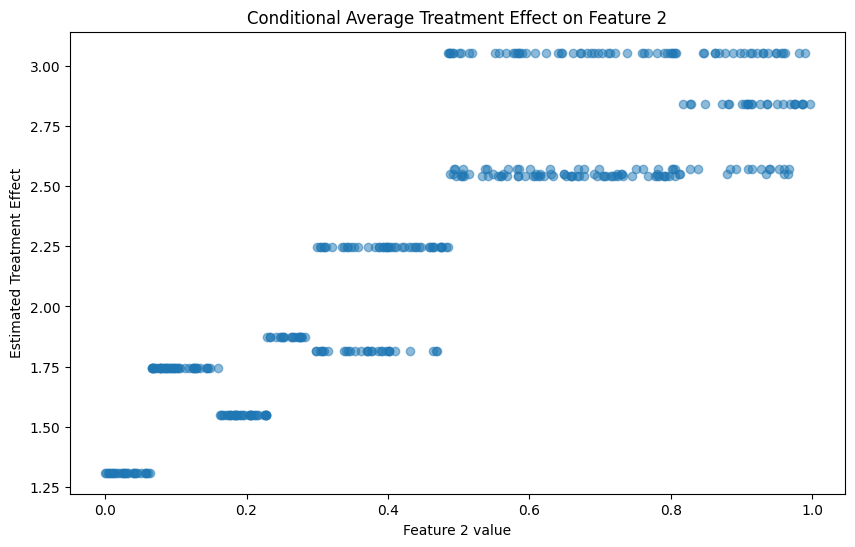
import numpy as np
import pandas as pd
from sklearn.model_selection import train_test_split

# 前回提供したCausalTreeNodeとCausalTreeクラスのコードをここに挿入してください

# サンプルデータの生成
def generate_sample_data(n_samples=1000, n_features=5):
    np.random.seed(42)
    X = np.random.rand(n_samples, n_features)

    # 処置の割り当て確率を共変量に基づいて決定
    propensity = 1 / (1 + np.exp(-(X[:, 0] + X[:, 1])))
    w = np.random.binomial(1, propensity)

    # 結果変数の生成
    y = 2 * X[:, 0] + 3 * X[:, 1] + w * (1 + 2 * X[:, 2]) + np.random.normal(0, 0.1, n_samples)

    return X, w, y

# データの生成
X, w, y = generate_sample_data(n_samples=2000)

# データの分割
X_train, X_test, w_train, w_test, y_train, y_test = train_test_split(X, w, y, test_size=0.2, random_state=42)

# Causal Treeモデルの構築
ct = CausalTree(max_depth=4, min_samples_leaf=100)
ct.fit(X_train, y_train, w_train)

# テストデータに対する予測
tau_pred = ct.predict(X_test)

# ATEの計算
def calculate_ate(model, X):
    tau_pred = model.predict(X)
    return np.mean(tau_pred)

ate = calculate_ate(ct, X_test)
print(f"Estimated ATE: {ate:.4f}")

# 真のATEの計算(この場合、データ生成プロセスを知っているため可能)
def true_effect(X):
    return 1 + 2 * X[:, 2]

true_ate = np.mean(true_effect(X_test))
print(f"True ATE: {true_ate:.4f}")

# ATTとATUの計算
def calculate_att_atu(model, X, w):
    tau_pred = model.predict(X)
    att = np.mean(tau_pred[w == 1])
    atu = np.mean(tau_pred[w == 0])
    return att, atu

att, atu = calculate_att_atu(ct, X_test, w_test)
print(f"Estimated ATT: {att:.4f}")
print(f"Estimated ATU: {atu:.4f}")

# 処置効果の異質性の可視化
import matplotlib.pyplot as plt

plt.figure(figsize=(10, 6))
plt.hist(tau_pred, bins=30, edgecolor='black')
plt.title('Distribution of Estimated Treatment Effects')
plt.xlabel('Estimated Treatment Effect')
plt.ylabel('Frequency')
plt.axvline(ate, color='red', linestyle='dashed', linewidth=2, label='ATE')
plt.axvline(att, color='green', linestyle='dashed', linewidth=2, label='ATT')
plt.axvline(atu, color='blue', linestyle='dashed', linewidth=2, label='ATU')
plt.legend()
plt.show()

# 特定の共変量に対する条件付き平均処置効果のプロット
feature_index = 2  # X[:, 2]に対する条件付き効果をプロット
plt.figure(figsize=(10, 6))
plt.scatter(X_test[:, feature_index], tau_pred, alpha=0.5)
plt.title(f'Conditional Average Treatment Effect on Feature {feature_index}')
plt.xlabel(f'Feature {feature_index} value')
plt.ylabel('Estimated Treatment Effect')
plt.show()
実行結果は以下のようになります。


Causal Forest
概念的説明
Causal Forestは、Causal Treeの概念を拡張し、より安定した処置効果の推定を実現する手法です。この手法の核心は、複数のCausal Treeを組み合わせることで、個々のツリーの不安定性や過学習の傾向を軽減することにあります。
Causal Forestのアルゴリズムは、ランダムフォレストの考え方を因果推論の文脈に適用したものと考えることができます。まず、元のデータセットからブートストラップサンプリングによって複数のサブセットを作成します。これにより、データの多様性を確保し、モデルの汎化性能を向上させます。次に、各サブセットに対して個別のCausal Treeを構築します。これらのツリーは、前回説明したCausal Treeのアルゴリズムに基づいて構築されますが、特徴量のランダムサブセットを使用することで、ツリー間の相関を減少させます。
CATE(Conditional Average Treatment Effect)の最終的な推定値は、全てのツリーの予測の平均として計算されます。この平均化プロセスにより、個々のツリーの予測の不確実性が軽減され、より安定した推定が可能になります。
アルゴリズムの詳細
Honest Splitting
Honest Splitting は、推定のバイアスを減少させるための重要な技術です。データを以下の 3 つのサブセットに分割します
Honest Splitting を使用する場合、CATE の推定は以下のように修正されます
Local Linear Forest
Local Linear Forest は、Causal Forest をさらに拡張し、各葉ノードで線形回帰を用いることでより柔軟なモデリングを実現します。CATE の推定は以下のように行われます
Causal Forestまとめ
Causal Forest は、個々の Causal Tree の不安定性を軽減しつつ、処置効果の異質性を捉える能力を維持します。また、特徴量の重要度や部分依存プロットなどの解釈手法を適用できる点も大きな利点です。ただし、無視可能性や重複などの仮定が満たされていることを確認し、結果の解釈には慎重を期す必要があります。
はてなブログで数式を書くとおかしくなる部分があるので、おかしい部分はすみません...
フルスクラッチ実装
class CausalTreeNode:
    def __init__(self, depth=0):
        self.feature_index = None  # 分割に使用する特徴量のインデックス
        self.threshold = None      # 分割の閾値
        self.tau = None            # 処置効果の推定値
        self.left = None           # 左の子ノード
        self.right = None          # 右の子ノード
        self.depth = depth         # ツリーにおける深さ
        self.parent = None         # 親ノードへの参照

class CausalTree:
    def __init__(self, max_depth=5, min_samples_leaf=10):
        self.root = None                     # ルートノード
        self.max_depth = max_depth           # 木の最大深さ
        self.min_samples_leaf = min_samples_leaf  # 葉ノードの最小サンプル数
        self.feature_importances_ = None     # 特徴量の重要度

    def fit(self, X, y, w):
        # モデルの学習を行う
        self.n_features = X.shape[1]  # 特徴量の数を保存
        self.feature_importances_ = np.zeros(self.n_features)  # 特徴量の重要度を初期化
        self.root = self._build_tree(X, y, w)  # 再帰的にツリーを構築

    def _build_tree(self, X, y, w, depth=0, parent=None):
        # 再帰的にツリーを構築する
        node = CausalTreeNode(depth)
        node.parent = parent

        # 停止条件: 最大深さに達した、またはサンプル数が最小値以下
        if depth == self.max_depth or len(y) <= self.min_samples_leaf:
            node.tau = self._estimate_tau(y, w)
            return node

        # 最適な分割点を見つける
        feature_index, threshold = self._find_best_split(X, y, w)

        if feature_index is None:
            # 分割できない場合は葉ノードとする
            node.tau = self._estimate_tau(y, w)
            return node

        # データを分割
        left_mask = X[:, feature_index] <= threshold
        right_mask = ~left_mask

        # ノードの情報を設定
        node.feature_index = feature_index
        node.threshold = threshold
        self.feature_importances_[feature_index] += 1  # 特徴量の重要度を更新

        # 子ノードを再帰的に構築
        node.left = self._build_tree(X[left_mask], y[left_mask], w[left_mask], depth + 1, node)
        node.right = self._build_tree(X[right_mask], y[right_mask], w[right_mask], depth + 1, node)

        return node

    def _find_best_split(self, X, y, w):
        # 最適な分割点を見つける
        best_feature = None
        best_threshold = None
        best_mse_reduction = 0

        for feature in range(self.n_features):
            thresholds = np.unique(X[:, feature])
            for threshold in thresholds:
                left_mask = X[:, feature] <= threshold
                right_mask = ~left_mask

                # 各子ノードのサンプル数が最小サンプル数以上であることを確認
                if np.sum(left_mask) < self.min_samples_leaf or np.sum(right_mask) < self.min_samples_leaf:
                    continue

                mse_reduction = self._calculate_mse_reduction(y, w, left_mask, right_mask)

                if mse_reduction > best_mse_reduction:
                    best_mse_reduction = mse_reduction
                    best_feature = feature
                    best_threshold = threshold

        return best_feature, best_threshold

    def _calculate_mse_reduction(self, y, w, left_mask, right_mask):
        # MSEの減少量を計算
        tau_parent = self._estimate_tau(y, w)
        tau_left = self._estimate_tau(y[left_mask], w[left_mask])
        tau_right = self._estimate_tau(y[right_mask], w[right_mask])

        mse_parent = np.mean((y - w * tau_parent) ** 2)
        mse_left = np.mean((y[left_mask] - w[left_mask] * tau_left) ** 2)
        mse_right = np.mean((y[right_mask] - w[right_mask] * tau_right) ** 2)

        n = len(y)
        n_left = np.sum(left_mask)
        n_right = np.sum(right_mask)

        return mse_parent - (n_left / n * mse_left + n_right / n * mse_right)

    def _estimate_tau(self, y, w):
        # 処置効果を推定
        treated = w == 1
        control = w == 0
        if np.sum(treated) == 0 or np.sum(control) == 0:
            return 0
        return np.mean(y[treated]) - np.mean(y[control])

    def predict(self, X):
        # 新しいデータに対して予測を行う
        return np.array([self._predict_single(x, self.root) for x in X])

    def _predict_single(self, x, node):
        # 単一のサンプルに対して予測を行う
        if node.left is None and node.right is None:
            return node.tau

        if x[node.feature_index] <= node.threshold:
            return self._predict_single(x, node.left)
        else:
            return self._predict_single(x, node.right)

class CausalForest:
    def __init__(self, n_estimators=100, max_depth=5, min_samples_leaf=10, subsample_ratio=0.8):
        self.n_estimators = n_estimators        # 木の数
        self.max_depth = max_depth              # 各木の最大深さ
        self.min_samples_leaf = min_samples_leaf  # 各木の葉ノードの最小サンプル数
        self.subsample_ratio = subsample_ratio  # サブサンプリングの比率
        self.trees = []                         # 木のリスト
        self.feature_importances_ = None        # 特徴量の重要度

    def fit(self, X, y, w):
        # モデルの学習を行う
        self.n_features = X.shape[1]
        self.feature_importances_ = np.zeros(self.n_features)

        # Honest splittingのためにデータを分割
        X_struct, X_est, y_struct, y_est, w_struct, w_est = train_test_split(
            X, y, w, test_size=0.5, random_state=42
        )

        for _ in range(self.n_estimators):
            # ブートストラップサンプリング
            n_samples = int(len(X_struct) * self.subsample_ratio)
            indices = np.random.choice(len(X_struct), n_samples, replace=True)
            X_boot, y_boot, w_boot = X_struct[indices], y_struct[indices], w_struct[indices]

            # 個々のCausal Treeを構築
            tree = CausalTree(max_depth=self.max_depth, min_samples_leaf=self.min_samples_leaf)
            tree.fit(X_boot, y_boot, w_boot)
            self.trees.append(tree)
            self.feature_importances_ += tree.feature_importances_

        # 特徴量の重要度を正規化
        self.feature_importances_ /= self.n_estimators

        # 推定用データセットを使用してτを再推定
        self._reestimate_tau(X_est, y_est, w_est)

    def _reestimate_tau(self, X, y, w):
        # 各木のτを再推定
        for tree in self.trees:
            self._reestimate_tau_tree(tree.root, X, y, w)

    def _reestimate_tau_tree(self, node, X, y, w):
        # 木のτを再帰的に再推定
        if node.left is None and node.right is None:
            mask = np.ones(len(X), dtype=bool)
            current = node
            while current.parent is not None:
                parent = current.parent
                if parent.left == current:
                    mask &= X[:, parent.feature_index] <= parent.threshold
                else:
                    mask &= X[:, parent.feature_index] > parent.threshold
                current = parent
            node.tau = self._estimate_tau(y[mask], w[mask])
        else:
            self._reestimate_tau_tree(node.left, X, y, w)
            self._reestimate_tau_tree(node.right, X, y, w)

    def _estimate_tau(self, y, w):
        # 処置効果を推定
        treated = w == 1
        control = w == 0
        if np.sum(treated) == 0 or np.sum(control) == 0:
            return 0
        return np.mean(y[treated]) - np.mean(y[control])

    def predict(self, X):
        # 新しいデータに対して予測を行う
        predictions = np.mean([tree.predict(X) for tree in self.trees], axis=0)
        return predictions
実際にサンプルデータで実行してみると
import numpy as np
from sklearn.model_selection import train_test_split
import matplotlib.pyplot as plt

# 上記で提供したCausalTreeNode, CausalTree, CausalForestクラスのコードをここに挿入してください

# サンプルデータの生成
def generate_sample_data(n_samples=1000, n_features=5):
    np.random.seed(42)
    X = np.random.randn(n_samples, n_features)

    # 処置の割り当て確率を共変量に基づいて決定
    propensity = 1 / (1 + np.exp(-(X[:, 0] + X[:, 1])))
    w = np.random.binomial(1, propensity)

    # 結果変数の生成
    y = 2 * X[:, 0] + 3 * X[:, 1] + w * (1 + 2 * X[:, 2]) + np.random.normal(0, 0.1, n_samples)

    return X, w, y

# データの生成
X, w, y = generate_sample_data(n_samples=2000)

# データの分割
X_train, X_test, w_train, w_test, y_train, y_test = train_test_split(X, w, y, test_size=0.2, random_state=42)

# Causal Forestモデルの構築
cf = CausalForest(n_estimators=100, max_depth=5, min_samples_leaf=10, subsample_ratio=0.8)
cf.fit(X_train, y_train, w_train)

# テストデータに対する予測
tau_pred = cf.predict(X_test)

# ATEの計算
ate = np.mean(tau_pred)
print(f"Estimated ATE: {ate:.4f}")

# 真のATEの計算(この場合、データ生成プロセスを知っているため可能)
def true_effect(X):
    return 1 + 2 * X[:, 2]

true_ate = np.mean(true_effect(X_test))
print(f"True ATE: {true_ate:.4f}")

# ATTとATUの計算
att = np.mean(tau_pred[w_test == 1])
atu = np.mean(tau_pred[w_test == 0])
print(f"Estimated ATT: {att:.4f}")
print(f"Estimated ATU: {atu:.4f}")

# 処置効果の異質性の可視化
plt.figure(figsize=(10, 6))
plt.hist(tau_pred, bins=30, edgecolor='black')
plt.title('Distribution of Estimated Treatment Effects')
plt.xlabel('Estimated Treatment Effect')
plt.ylabel('Frequency')
plt.axvline(ate, color='red', linestyle='dashed', linewidth=2, label='ATE')
plt.axvline(att, color='green', linestyle='dashed', linewidth=2, label='ATT')
plt.axvline(atu, color='blue', linestyle='dashed', linewidth=2, label='ATU')
plt.legend()
plt.show()

# 特定の共変量に対する条件付き平均処置効果のプロット
feature_index = 2  # X[:, 2]に対する条件付き効果をプロット
plt.figure(figsize=(10, 6))
plt.scatter(X_test[:, feature_index], tau_pred, alpha=0.5)
plt.title(f'Conditional Average Treatment Effect on Feature {feature_index}')
plt.xlabel(f'Feature {feature_index} value')
plt.ylabel('Estimated Treatment Effect')
plt.show()

# モデルの性能評価(MSE)
mse = np.mean((y_test - (w_test * tau_pred + (1 - w_test) * 0)) ** 2)
print(f"Mean Squared Error: {mse:.4f}")

# 特徴量の重要度(簡易版)
feature_importances = np.zeros(X.shape[1])
for tree in cf.trees:
    feature_importances += tree.feature_importances_
feature_importances /= len(cf.trees)

plt.figure(figsize=(10, 6))
plt.bar(range(X.shape[1]), feature_importances)
plt.title('Feature Importances')
plt.xlabel('Feature Index')
plt.ylabel('Importance')
plt.show()
実行結果は以下です


最後に
今回は、私もかなり気になっていた、CATEを算出する手法、Causal Treeとその進化版Causal Forestに関して、理論とフルスクラッチ実装の解説を行ってみました。私が、本当に記事を書きたかったのはこの部分で、記事を書くことを口実に勉強をちゃんとしたかった部分でもあります。最近は、meta-learnerが波に乗っていて、Causal TreeやCausal Forestを使用した実例などは聞きませんが、meta-learnerと同様に、CATEを算出する手法という意味で大変興味を持っていた手法でした。現状の書籍などで、きちんと理論やフルスクラッチ実装に触れているものはなかったはずなので、どなたかの参考になれば幸いです。因みにCausal TreeやCausal Forestはhold-out推奨ですからね!
ただ恐らく、一部数式がはてなブログのせいで、上手く表示できてないor間違っている部分があるので、気を付けてお読みいただければと思います。因果推論の分野はやはり面白いですね!